This article describes the workflow for performing a simple multiphysics analysis on the Nimbix platform using COMSOL® software. COMSOL® software package offers the capabilities of performing heat transfer, electromagnetic, structural analysis, and multiphysics analysis either as stand-alone or using a high-performance cloud computing service such as the one offered by NIMBIX. The case study presented in this article will be demonstrating the COMSOL® workflow on Nimbix using COMSOL® release 5.5.
To perform heat transfer analysis using COMSOL® on Nimbix cloud computing, the following steps can be followed (for detailed instructions on using COMSOL®, consult COMSOL® user manuals and tutorials):
1. Select Compute from your NIMBIX account menu (the “All Apps” window will be displayed in your browser and all the NIMBIX cloud supported software will be shown). Start COMSOL® software by clicking on the COMSOL® 5.5 icon, as shown below.
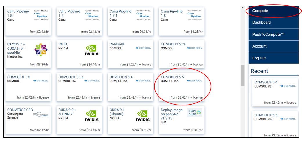
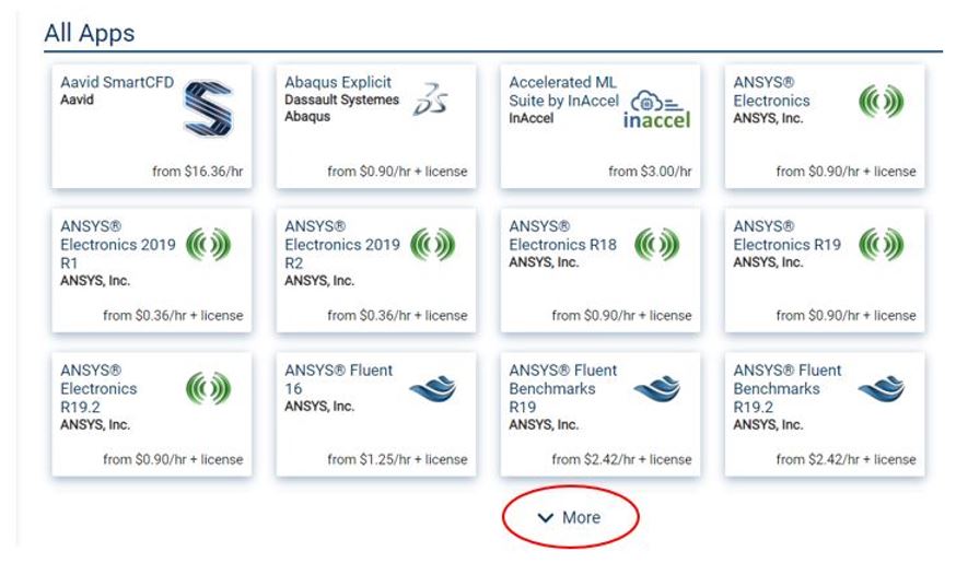
NOTE: If the option (for example latest COMSOL release or any other release) is not available in the first-page menu, click on “More” at the bottom of the page as shown in the image below:
2. A splash window will open. Select the COMSOL® 5.5 (or any other release you prefer) option as shown below:
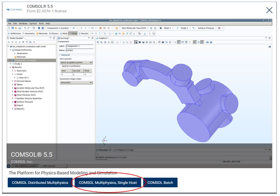
NOTE: For the example presented in this article (simple heat transfer problem), COMSOL Multiphysics, Single Host will be selected. Single host option allows you to choose either an “n” or and “NC” computer with the specified number of cores (use practical judgment when selecting the number of cores based on cost vs. performance needs). When running interactive based applications, you’ll find that choosing an NC9 or any NC* machine types should offer significant visual performance over not selecting an NC machine type. By choosing an NC machine, this places a GPU on your head-node and provides better visual performance. Another thing to keep in mind is that when running interactively, you can use a web browser, or in some cases for large models, or you might consider using RealVNC.
NOTE: For complex problems that require more computing power, use the “COMSOL Distributed Multiphysics” option. This will allow the user to select more nodes to decrease computation time and improve efficiency. The required NIMBIX “nodes.txt” file is automatically passed by NIMBIX to the head node, so no additional input is necessary to distribute the job across multiple nodes.
3. The cloud set-up screen opens, and here you must choose some of your settings by clicking on the Tabs on the top of the window (General, Optional, etc.) one tab at a time, starting with GENERAL.
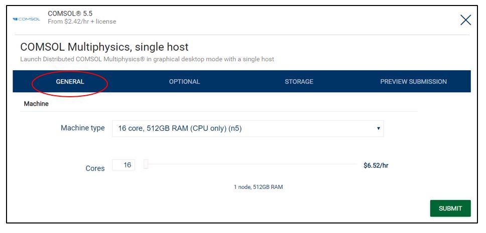
UNDER GENERAL TAB
1. Under Machine type drop down menu, when clicked, you have the choice of selecting the type of machine you want to run your job on. The decision on machine type selection is based on the size and complexity of your model and cost associated with the machine type (some machines will have higher RAM, others will only run the job on single CPU, others will have better graphics and therefore higher cost, etc.).
For the example presented here, we selected 16 core machine with 512GB RAM.
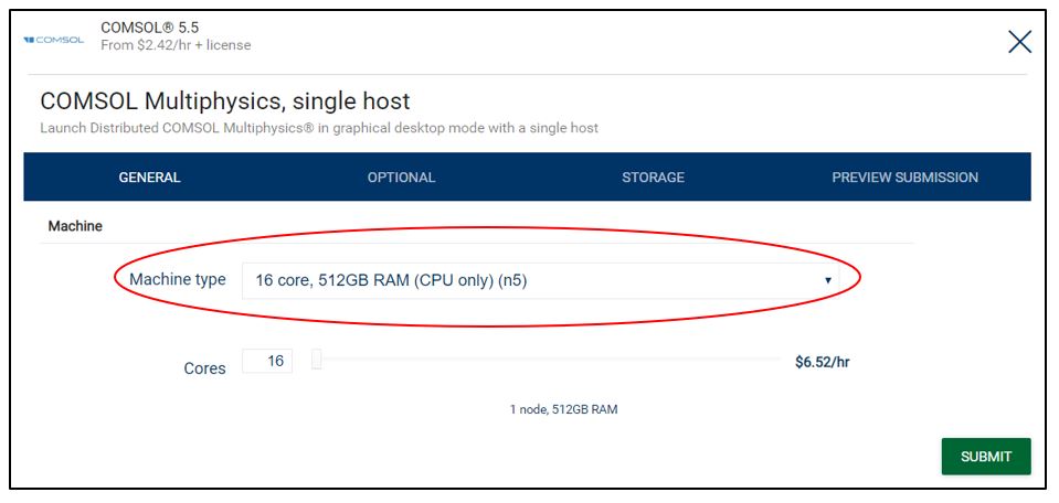
NOTE: Because the single host option was selected, it is not possible to increase the number of cores since this would use more than a single host. The Default “1 node” 512GB RAM pops up, and the number of nodes cannot be changed. The machine type you selected in this step will dictate the number of cores allocated. Do not mistake the number of cores with the number of nodes (nodes represent the number of increment of cores that you selected. In the example above, 1 node represents 16 cores, 2 nodes represent 32 cores).
UNDER OPTIONAL TAB
1. Assign a JOB LABEL (give a name that will help you keep track of your running jobs. For example, MyFreeConvProblem):
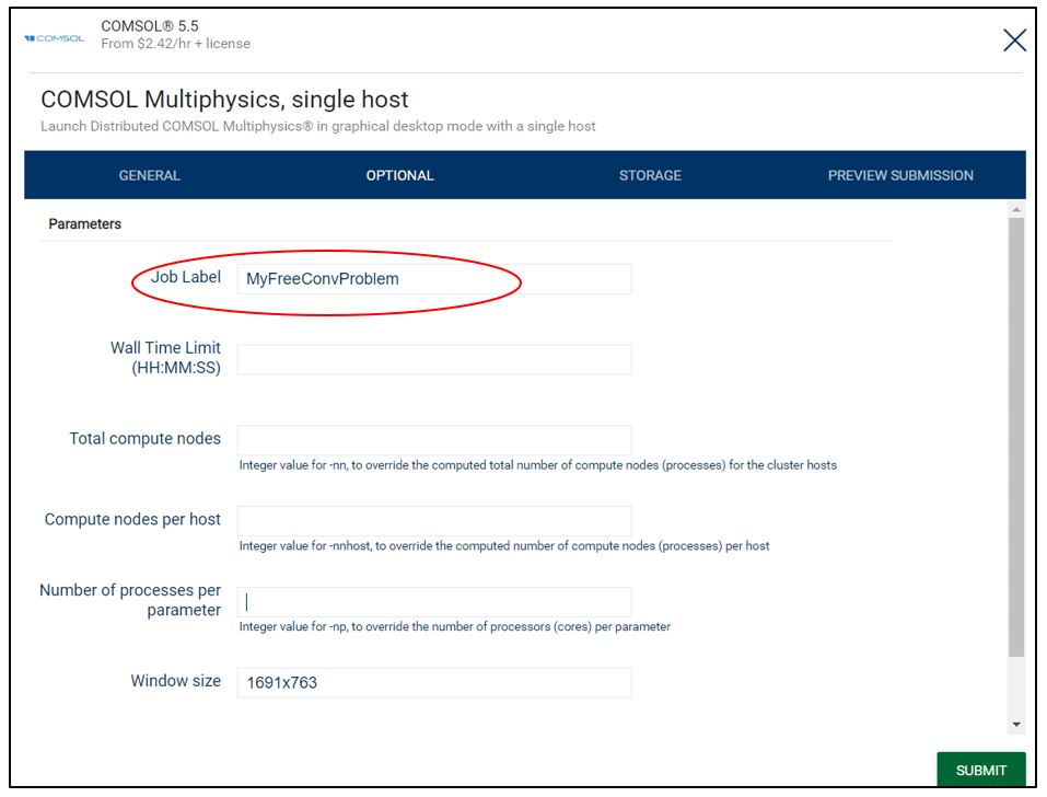
NOTE: Unless you have all the other information to fill in all other boxes such as “Total compute nodes” or “Compute nodes per host”, etc., you can leave them blank and move on to the next Tab. These options are used to overwrite the default settings based on the selection in the “General” tab.
UNDER STORAGE TAB
1. Select vault type: Default vault is “Elastic_File”.

The “Elastic_File” vault is recommended for small to medium size jobs, such as Icepak projects, simple linear Mechanical Analysis projects, some HFSS and simple Fluent projects (not multi-phase). For any complex and computationally heavy jobs, and where partitioning the job over number of cores becomes challenging, the Performance_SSD vault is strongly recommended. The Performance_SSD vault can be found in the drop-down under “Select Vault” tab (NOTE: requires subscription and extra monthly payment to have access to Performance_SSD vault).
Before submitting your job for running, you can preview your settings under the PREVIEW SUBMISSION tab.
COMSOL CONVECTION HEAT TRANSFER PROBLEM (MULTIPHYSICS) SETUP WORKFLOW
Here are the steps for setting up and solving a 2D CFD/heat transfer multiphysics problem on NIMBIX cloud using COMSOL® 5.5 software (Model Wizard was used for setting up this problem):
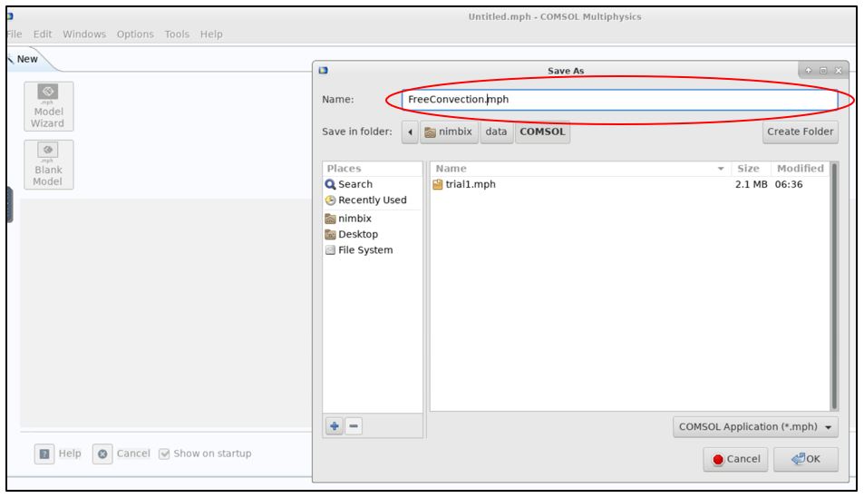
1. Start by saving your model to avoid losing your work in case of a network outage (recommend saving as often as you complete important problem steps to avoid losing your work). Provide a name (try and keep it simple and, if possible, do not leave blank space between words) that is representative of the physics of the problem. For this example, we named the project “FreeConvection”:
 2. Under New window, click on the Model Wizard. Once it opens, select 2D.
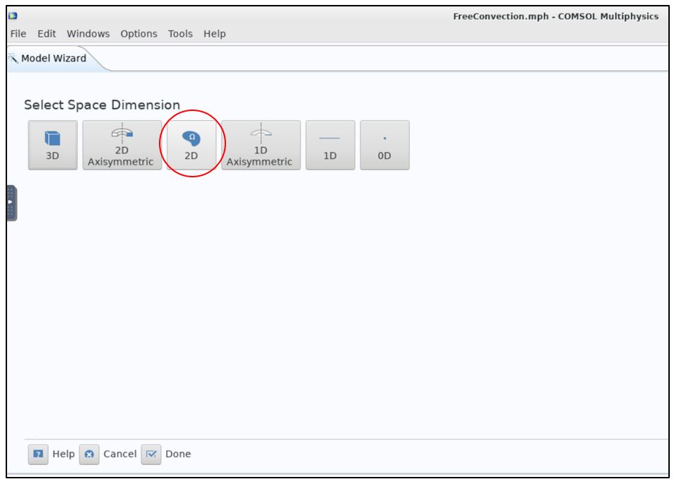
3. Once you click on the 2D space dimension, the “Model Wizard” window will open:
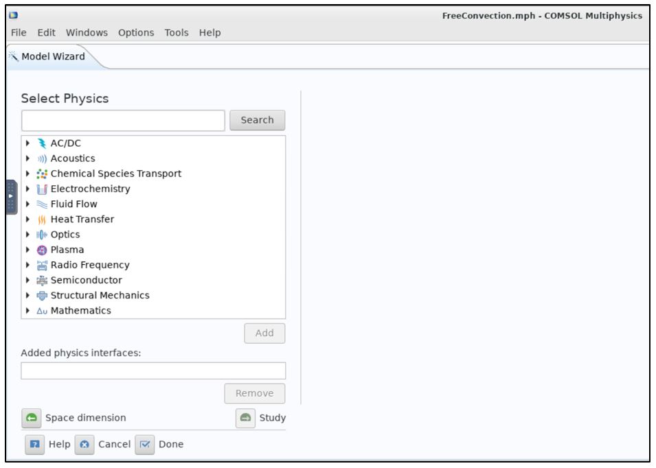
4. Under Select Physics option, select Fluid Flow to Single-Phase Flow to Laminar Flow (spf):
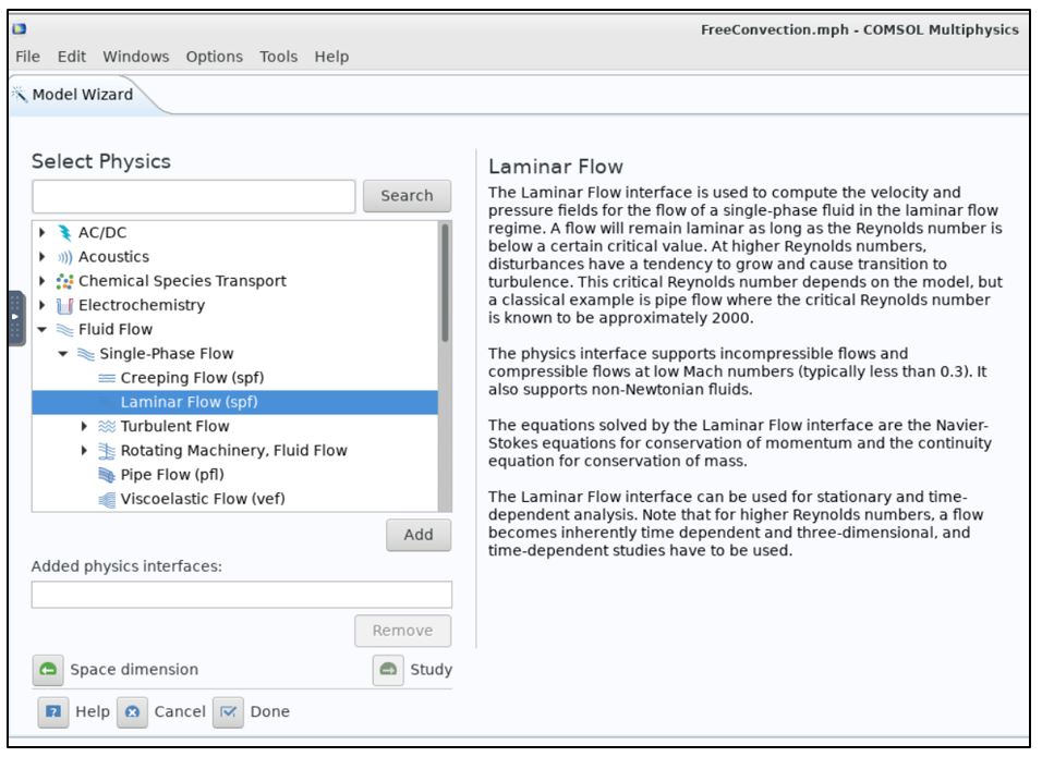
5. Click “Add” button to add the laminar flow physics to the problem.
6. Under Select Physics, click on Heat Transfer and select Heat transfer in Fluids (ht) as shown below:
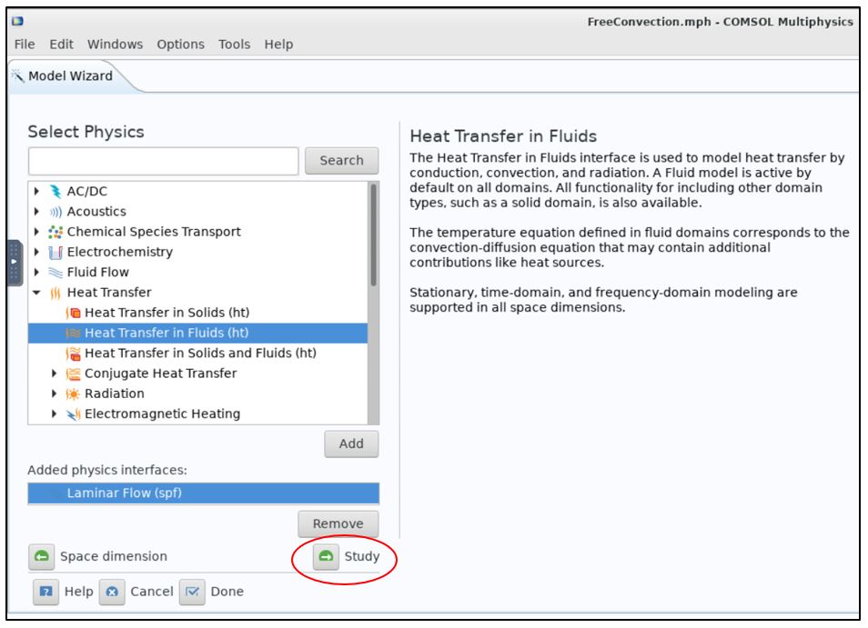
7. Click the “Add” button to add the heat transfer in fluids physics to the problem to be solved.
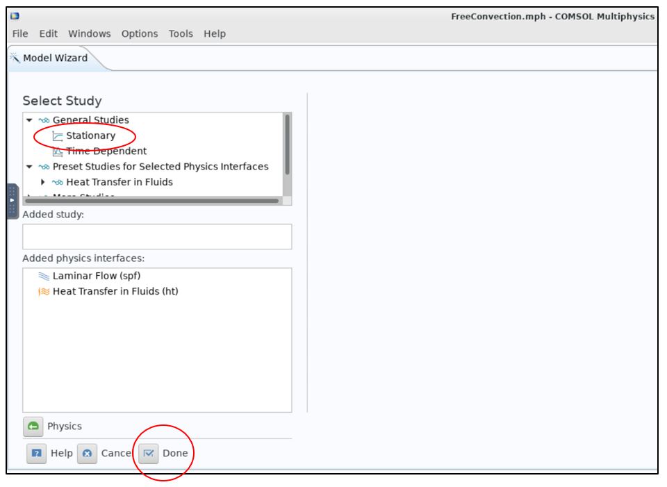
8. Click on the “Study” button and, under Select Studies option, select the “Stationary” option from General Studies drop down options, as shown below. Click the “Done” button to complete the wizard set-up.
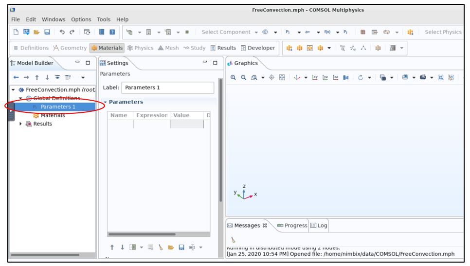
9. At this point, we are ready to assign material properties, parameters or equations for inlet, outlet boundary conditions, etc. Under “Model Builder” view, click on the “Global Definitions” and select “Parameters 1: as shown below(graphics window may differ in some cases):
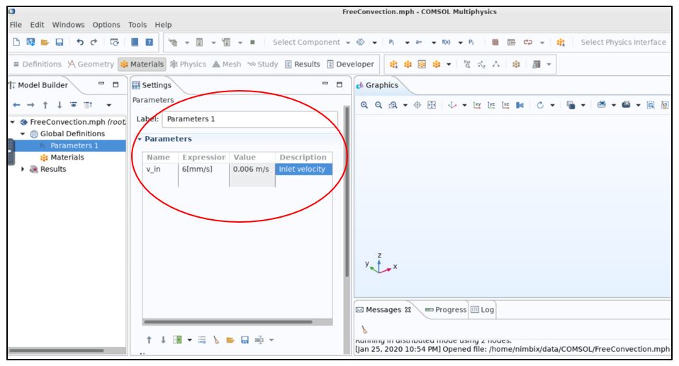
10. In the Parameters settings window, under “Parameters,” enter the settings for inlet velocity, as shown below:
11. Following the same steps, add additional parameters for boundary conditions (as seen in the image below):

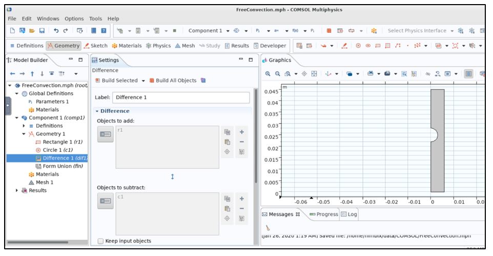
12. In the next step, we will start building the geometry, which is going to be a simple 2D geometry with a small circular cut-out (use symmetry as much as possible to simplify your model), as shown below:
13. Set-up your Multiphysics analysis (laminar flow and heat transfer inlet, outlet, and boundary conditions).
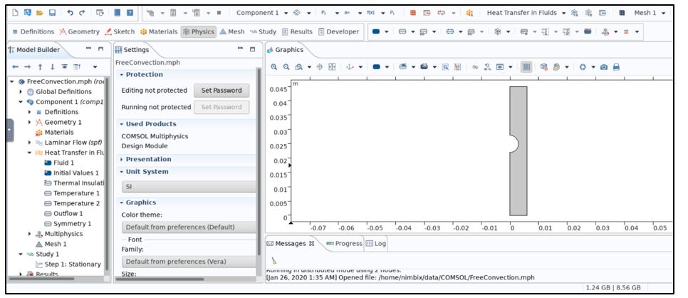
NOTE: Multiphysics model is all set-up at this point and is ready for meshing.
14. Mesh your computational domain: right-click on the “Mesh 1” and select “Build All” from the flyout menu.
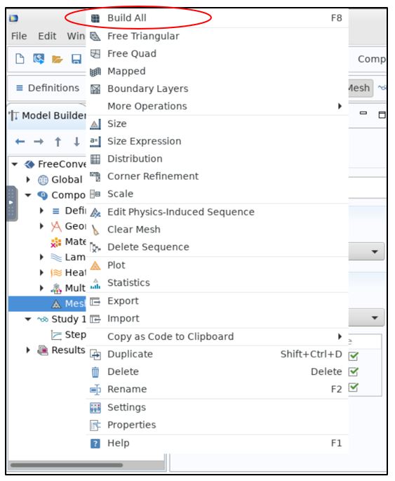
NOTE: Use the “Build All” option for default mesh settings or refine your mesh as desired.
15. Add Materials to your model. In this case, we added a material from the built-in materials library by right-clicking on Materials to Add Material from Library. Select “Water Fluid” from the built-in material library for this example.
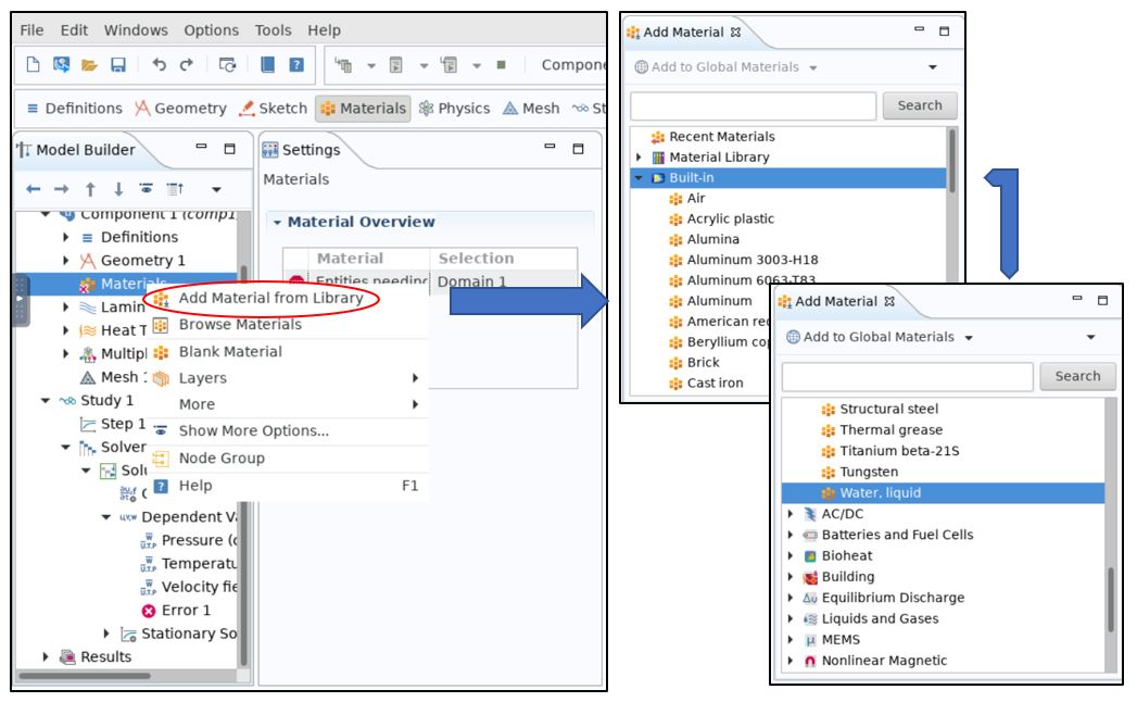
Note: The “Add Material” window opens on the right-hand side of your model window.
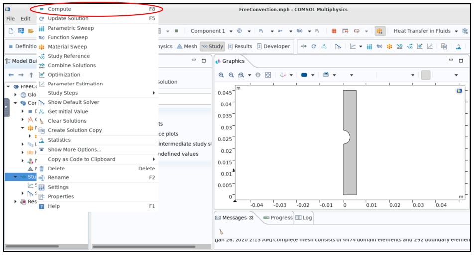
16. Run your model. Right-click on Study in the Model Builder tree and select “Compute” option from the fly-out menu:
Note: The “Add Material” window opens on the right-hand-side of your model window.
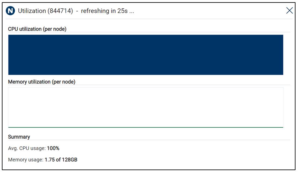
17. Monitor your CPU utilization (Click “Detailed Job Metrics” to see the utilization of your nodes during Solve):
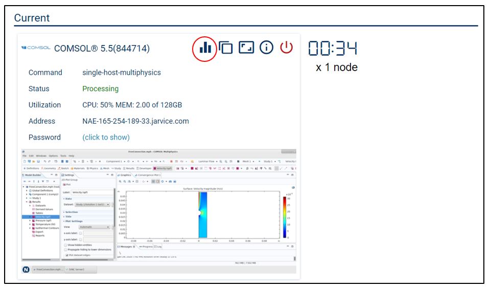
NOTE: The CPU utilization time refreshes every 30 seconds. For distributed problems, all nodes will be displayed along with CPU utilization per node.
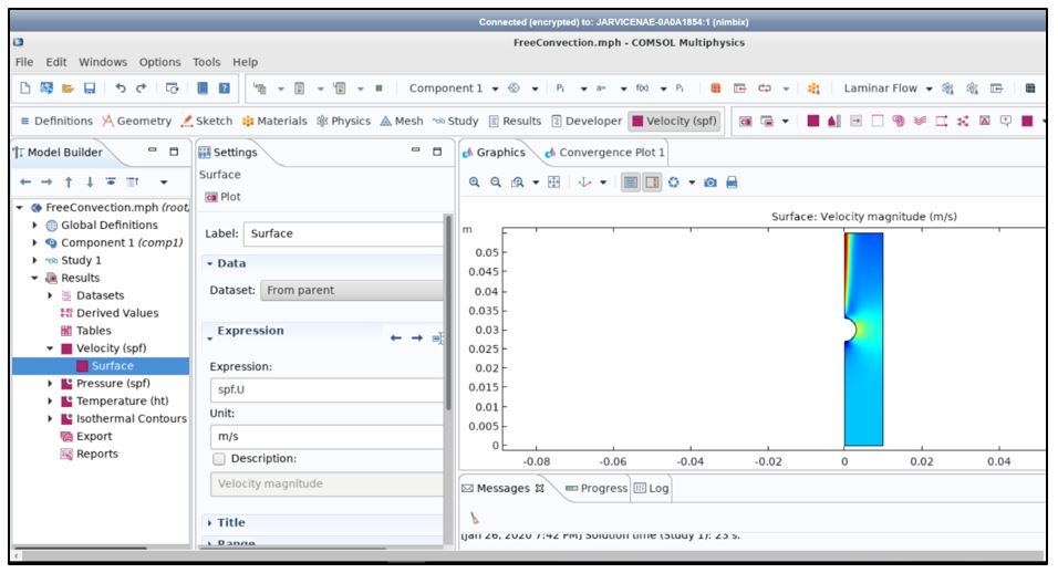
18. Insert and review your results (select results as desired in the “Model Builder” view/tab under “Results”) as shown below:
19. Save and Exit once post-processing is completed.
NOTE: COMSOL® software is a general-purpose FEM software (much as like ANSYS FEA software suite) that offers several features that can make it more palatable to users than advanced ANSYS options
- Ability to solve multiple problems using the same graphical user interface (all-in-one Multiphysics analysis options)
- Customizable (more oriented towards academia than industry – like ANSYS)
- Available on NIMBIX cloud using high-performance computing platform
- Excellent tutorial and training materials that can be easily accessed from the web