This article describes the workflow for performing a simple multiphysics analysis on the Nimbix platform using COMSOL® software. COMSOL® software package offers the capabilities of performing heat transfer, electromagnetic, structural analysis, and multiphysics analysis either as stand-alone or using a high-performance cloud computing service such as the one offered by Nimbix. The case study presented in this article will demonstrate the COMSOL® workflow on Nimbix using COMSOL® Release 5.5 available on Nimbix.
To perform heat generation in a vibrating structure analysis using COMSOL® on Nimbix cloud computing, the following steps can be followed (for detailed instructions on using COMSOL®, consult COMSOL® user manuals and tutorials):
1. Select Compute from your Nimbix account menu (the “All Apps” window will be displayed in your browser, and all the NIMBIX cloud supported software will be shown). Start COMSOL® software by clicking on the COMSOL® 5.5 icon, as shown below.
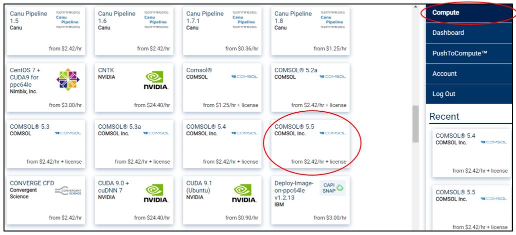
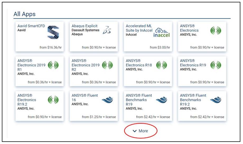
NOTE: If the option (for example latest COMSOL release or any other release) is not available in the first-page menu, click on “More” at the bottom of the page as shown in the image below:
2. After you clicked on COMSOL® 5.5 (or any other release you prefer), a splash window will open. Select the option of COMSOL Distributed Multiphysics, as shown below:
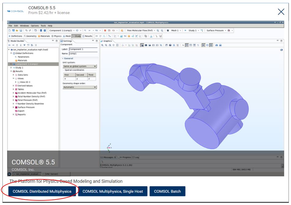
NOTE: For the fairly complex example that will be presented in this article (heat generation in a vibrating structure), COMSOL Distributed Multiphysics is selected. This will allow the user to select more nodes to decrease computation time and improve efficiency. The required NIMBIX “nodes.txt” file is automatically passed by NIMBIX to the head node, so no additional input is needed to distribute the job across multiple nodes.
COMSOL Distributed Multiphysics option allows the user to select either an “N” or and “NC” computer with the specified number of cores (use practical judgment when selecting the number of cores based on cost vs. performance needs). When running interactive based applications, you’ll find that selecting an NC9 or any NC* machine types should offer significant visual performance over not selecting an NC machine type. By selecting an NC machine, this places a GPU on your head-node and offers better visual performance. Another thing to keep in mind is that when running interactively you can use a web browser, or in some cases for large models, or you might consider using RealVNC.
3. The cloud set-up screen opens, and here you must choose some of your settings by clicking on the Tabs on the top of the window (General, Optional, etc.) one tab at a time, starting with GENERAL.
UNDER GENERAL TAB
1. Under Machine type fly-down, when clicked, you have the choice of selecting the type of machine you want to run your job on. The decision on machine type selection is based on the size and complexity of your model and cost associated with the machine type (some machines will have higher RAM, others will only run the job on single CPU, others will have better graphics and therefore higher cost, etc.).
For the example presented here, we selected 16 core Machine with 512GB RAM (2 nodes).
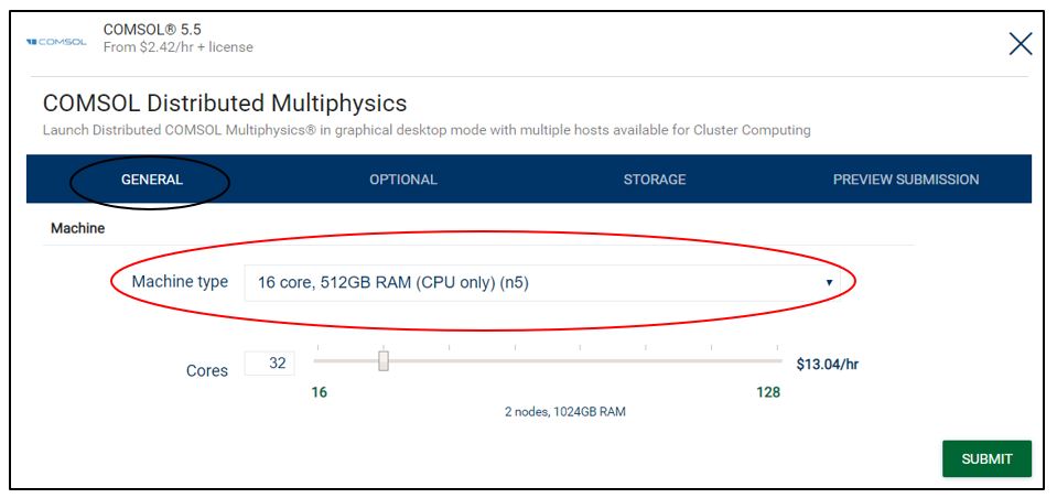
2. To decrease the computational time, choose the number of cores that you believe are needed (depending on the complexity of the problem). For the example presented in this article, we will select 32 cores, which is equivalent to 2 nodes (of 16 cores each):
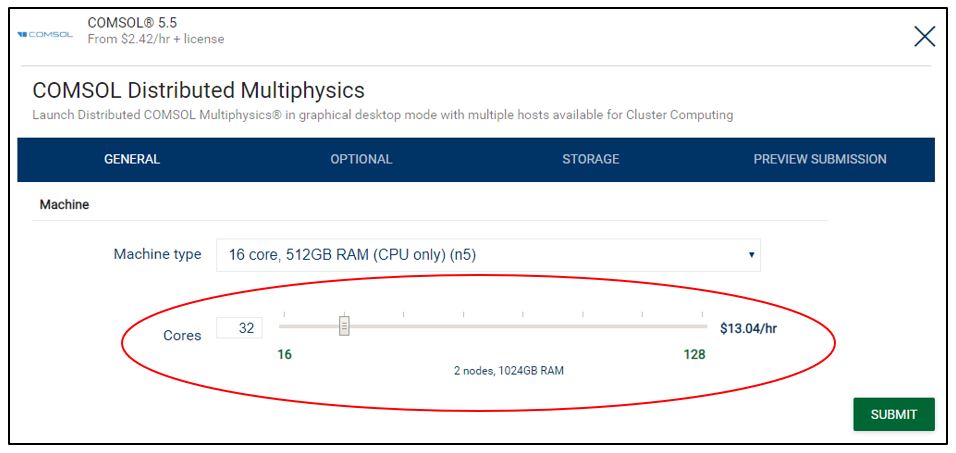
NOTE: The machine type you selected in the previous step, will dictate the number of cores allocated. Do not mistaken the number of cores with the number of nodes (nodes represent the number of increment of cores that you selected. In the example above, 1 node represents 16 cores, 2 nodes represent 32 cores). You can adjust the number of cores to whatever number you want by simply typing over the default “16” next to the Cores box, the number of cores (in this case “32”), and hit Return to accept it.
UNDER OPTIONAL TAB
1. Assign a JOB LABEL (give a name that will help you keep track of your running jobs. For example, MyHeatGenVibratStruct):
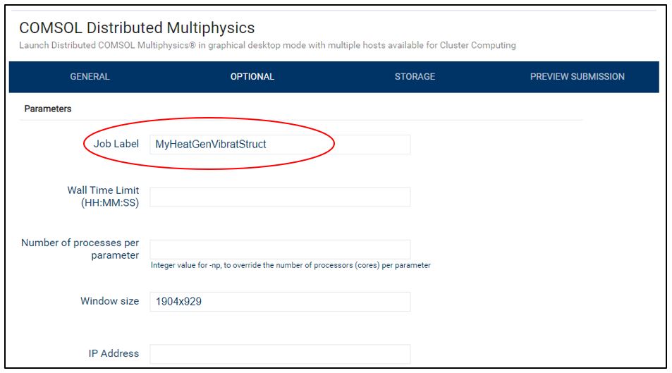
NOTE: Unless you have all the other information to fill in all other boxes such as “Number of processes per parameter,” etc., you can leave them blank and move on to the next Tab. These options are used to overwrite the default settings based on the selection in the “General” tab.
UNDER STORAGE TAB
1. Select vault type: Default vault is “Elastic_File”

The “Elastic_File” vault is recommended for small to medium size jobs, such as Icepak projects, simple linear Mechanical Analysis projects, some HFSS and simple Fluent projects (not multi-phase). For any complex and computationally heavy jobs, and where partitioning the job over number of cores becomes challenging, the Performance_SSD vault is strongly recommended. The Performance_SSD vault can be found in the drop-down under “Select Vault” tab (NOTE: requires subscription and extra monthly payment to have access to Performance_SSD vault).
Before submitting your job for running, you can preview your settings under the PREVIEW SUBMISSION tab.
COMSOL THERMAL STRUCTURE INTERACTION PROBLEM (MULTIPHYSICS) SETUP WORKFLOW
Here are the steps for setting up and solving a 3D thermal-structure interaction Multiphysics problem on NIMBIX cloud using COMSOL® 5.5 software (Model Wizard was used for setting up this problem):
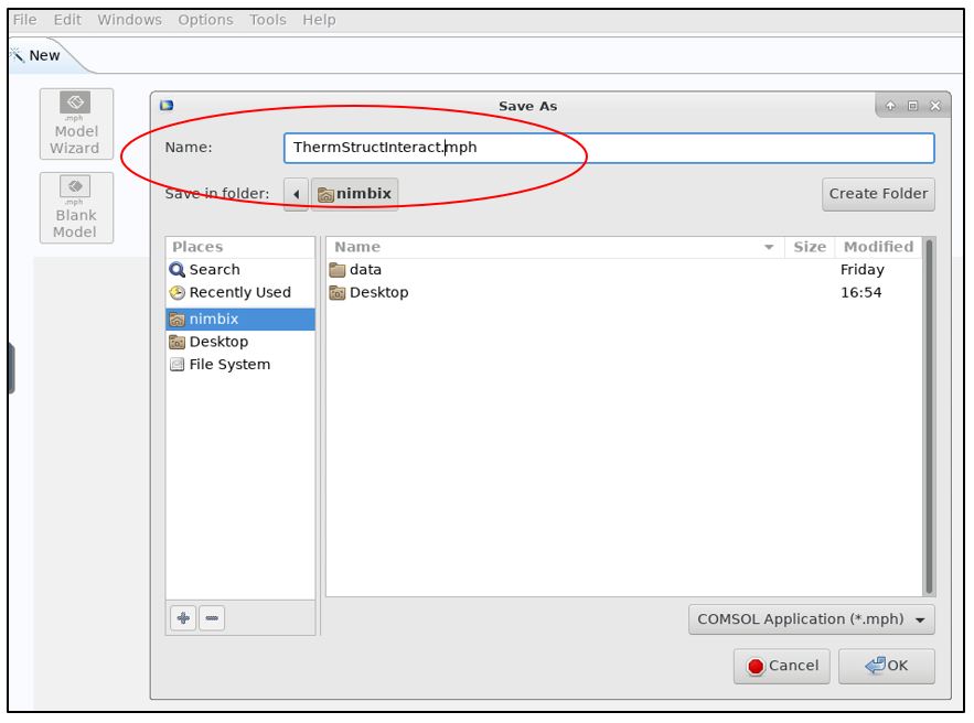
1. Start by saving your model to avoid losing your work in case of a network outage (recommend saving as often as you complete important problem steps to avoid losing your work). Provide a name (try and keep it simple and, if possible, do not leave blank space between words) that is representative of the physics of the problem. For this example, we named the project “ThermStructInteract”:
2. Under New window, click on the Model Wizard. Once it opens, select 3D.
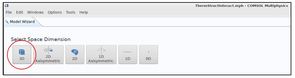
3. Once you click on the 3D space dimension, the “Model Wizard” window will open:
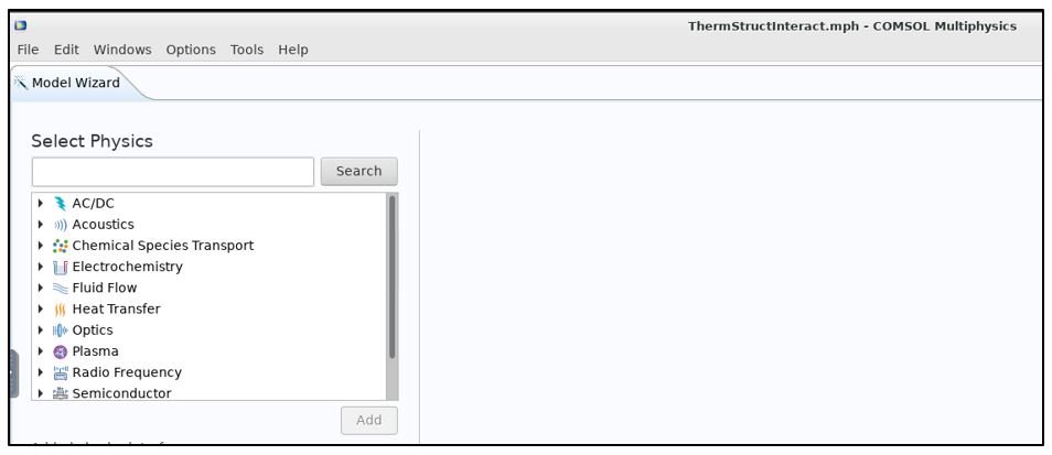
4. Under Select Physics option, select Heat Transfer à Heat Transfer in Solids (ht):
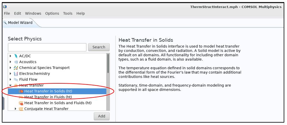
5. Click the “Add” button to add the heat transfer in solids physics to the problem.
6. Under Select Physics option, click on Structural Mechanics and select Solid Mechanics (solid) as shown below:
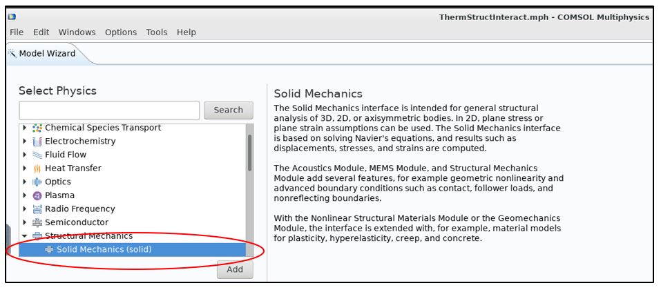
7. Click the “Add” button to add the Solid Mechanics physics to the problem to be solved.
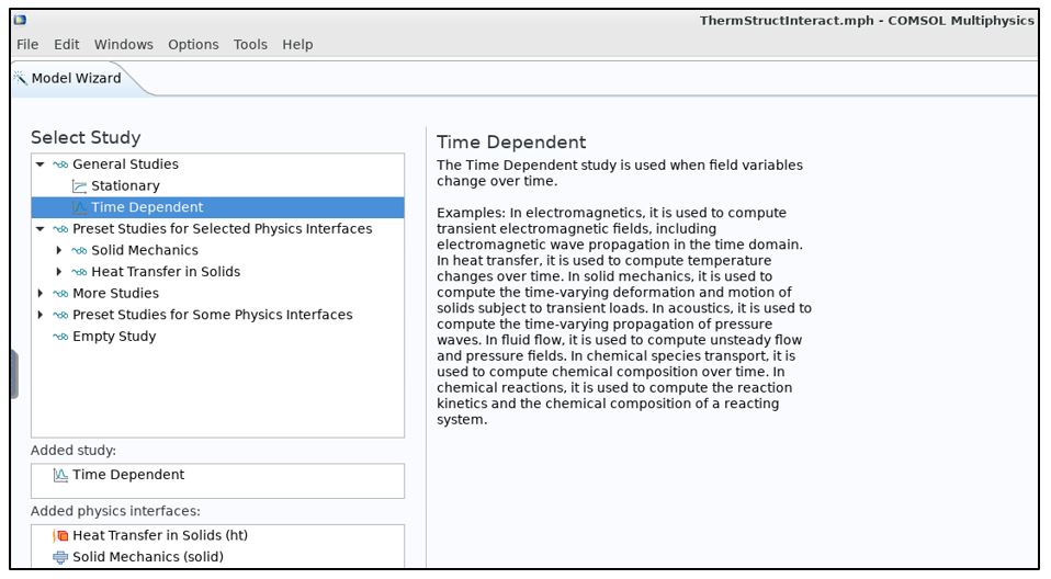
8. Click on the “Study” button and select General Studies to Time Dependent option, as shown below. Click the “Done” button to complete the wizard set-up.
9. At this point, we are ready to build the geometry that we wish to analyze. In the Geometry toolbar, click Block, as shown below:
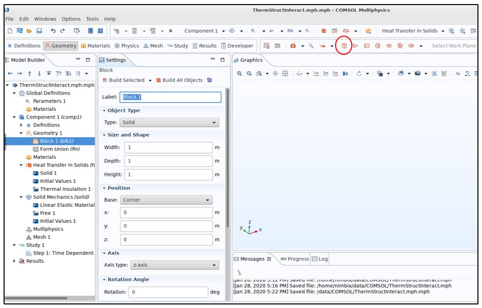
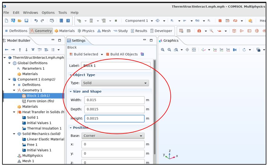
10. In the Settings window, under “Size and Shape” section, enter the settings for first block geometry, as shown below:
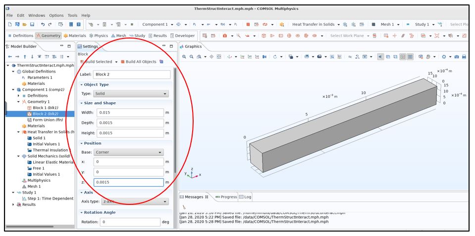
11. Following the same steps, build/add a second Block geometry (as seen in the image below):
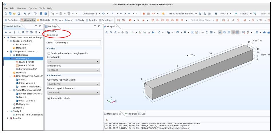
12. In the Model Builder, click Geometry I and click Build All objects as shown below:
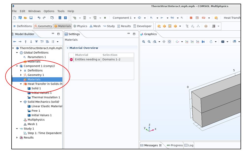
13. In the next step, we will add material from the Material Library by clicking on the Home toolbar and Materials, as shown below:
14. Go to Add Materials button from the Materials toolbar and select Built-in to Aluminum, as shown below:
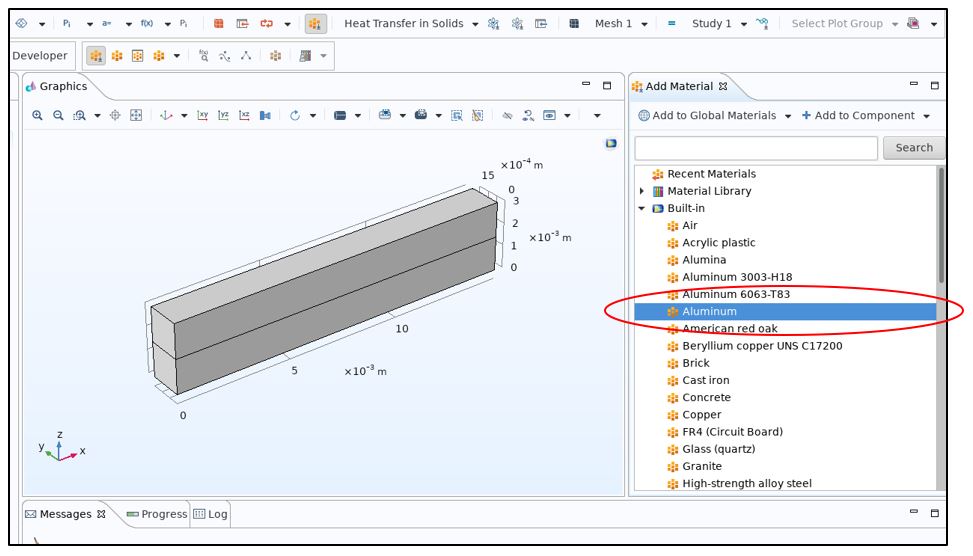
15. Click Add to Component.
16. Following the same steps as in Step 14, select Built-in to Magnesium AZ31B.
17. Click Add to Component again.
18. Close Materials toolbar by clicking Add Material window.
19. Under Model Builder, click Component 1 to Materials and select Aluminum (mat 1) and select Domain 1 under the Selection, as shown below:
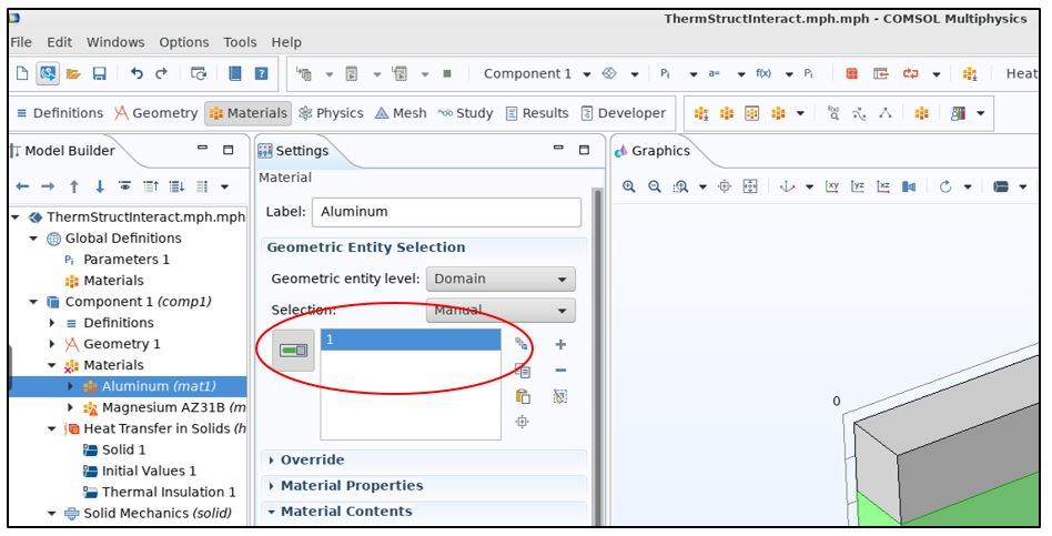
20. Similarly, under Model Builder, click Component 1, select Magnesium AZ31B, and choose Domain 2.
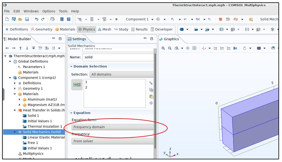
21. Set up Solid Model Equation Form to Frequency domain, since we plan on choosing the study type as Time Dependent. The time-dependent (transient) equation will apply only to the heat transfer physics. Go to Model Builder to Component 1 (comp 1) and click Solid Mechanics (solid).
22. In the Settings window, click Equation to expand, and under Equation Form choose Frequency domain, as shown below:
23. From Frequency list choose User Defined (we will define a user-defined function):
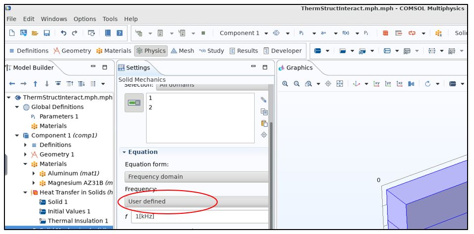
24. Type 8500 under the “f” text field.
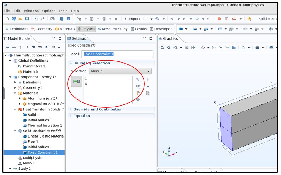
25. Assign boundary conditions (loads and constraints) by clicking on the Physics toolbar.
26. Under the Physics toolbar, click Boundaries and choose Fixed Constraint. Select boundaries 1 and 4, as shown below:
27. Under the Physics toolbar, click Boundaries and choose Boundary Load. Select boundaries 10 and 11, as shown below:
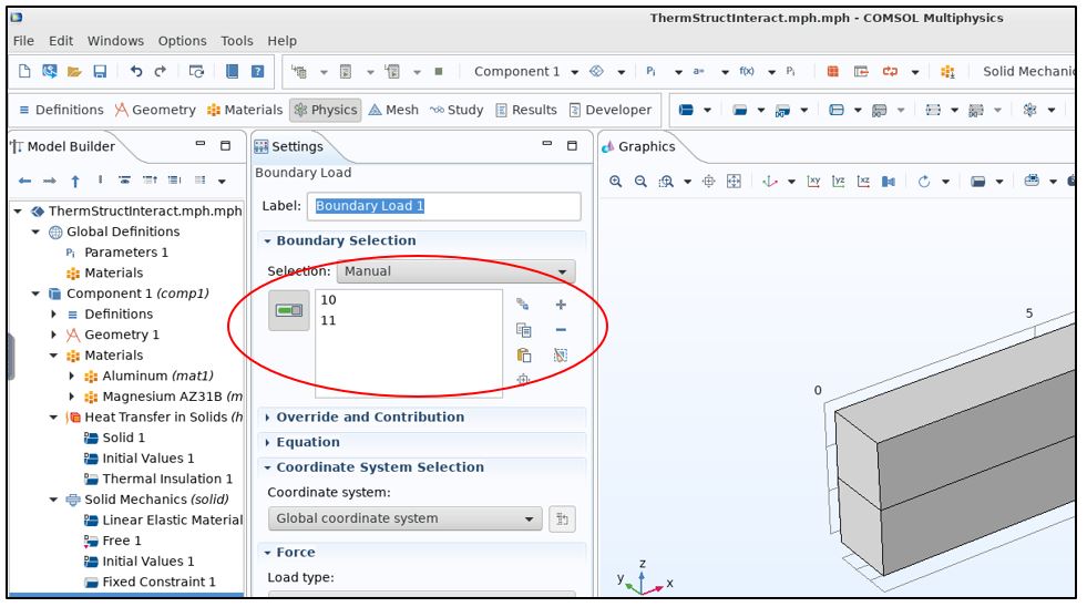
28. Under Boundary Load to Force section, type 2.25 [MPa] under z vector. Leave all other values default.
29. Under Model Builder to Solid Mechanics (solid), select Linear Elastic Material 1.
30. In the Physics toolbar, click Attributes and select Damping as shown below:
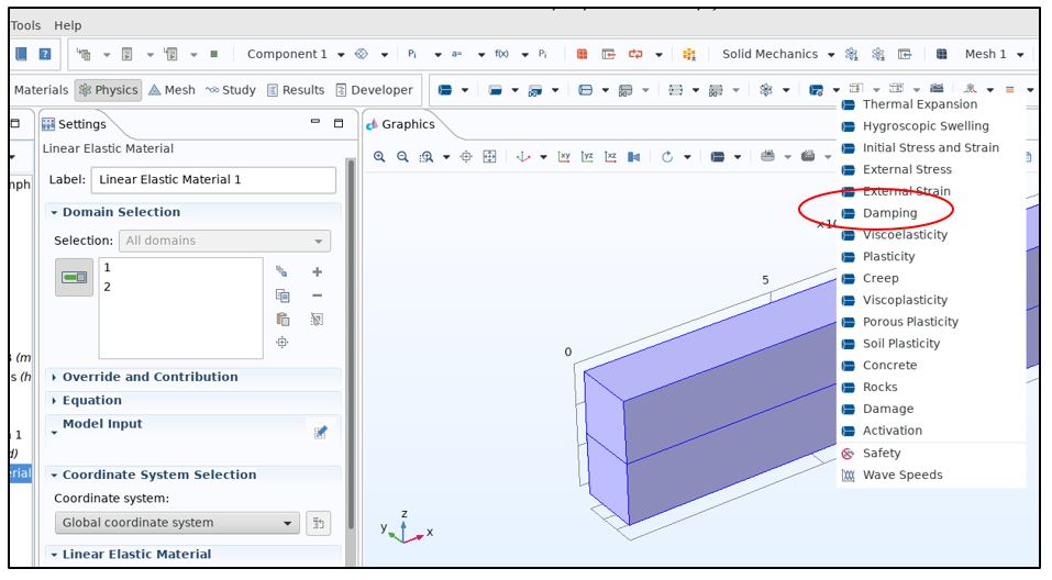
31. Select Domain 2.
32. Under Damping settings, select Isotropic loss factor and select User Defined, under the Isotropic loss list. Type 0.004 in the text file.
33. In the Model Builder, under Component 1, click Heat Transfering solids (ht).
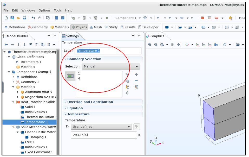
34. In the Physics toolbar click Boundaries and choose Temperature and select Boundaries 1 and 4, as shown in the image below:
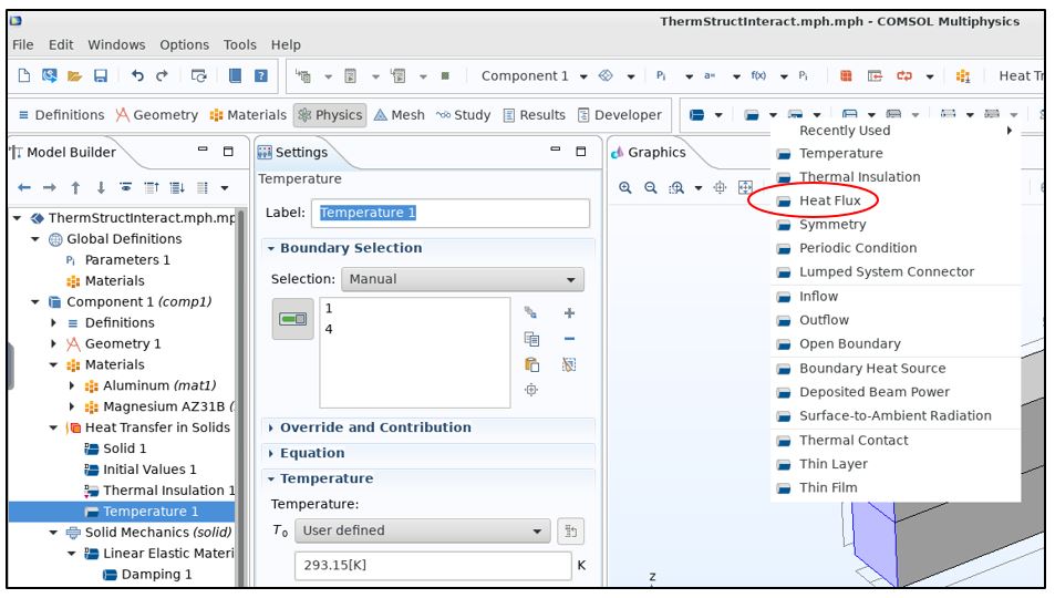
35. In the Physics toolbar, under Boundaries, select Heat Flux, as shown below:
36. Under heat flux, click Convective heat flux and under “h” value text field, type 6 (this defines the heat transfer coefficient).
37. Select boundaries 2,3,5 and 7 to 9.
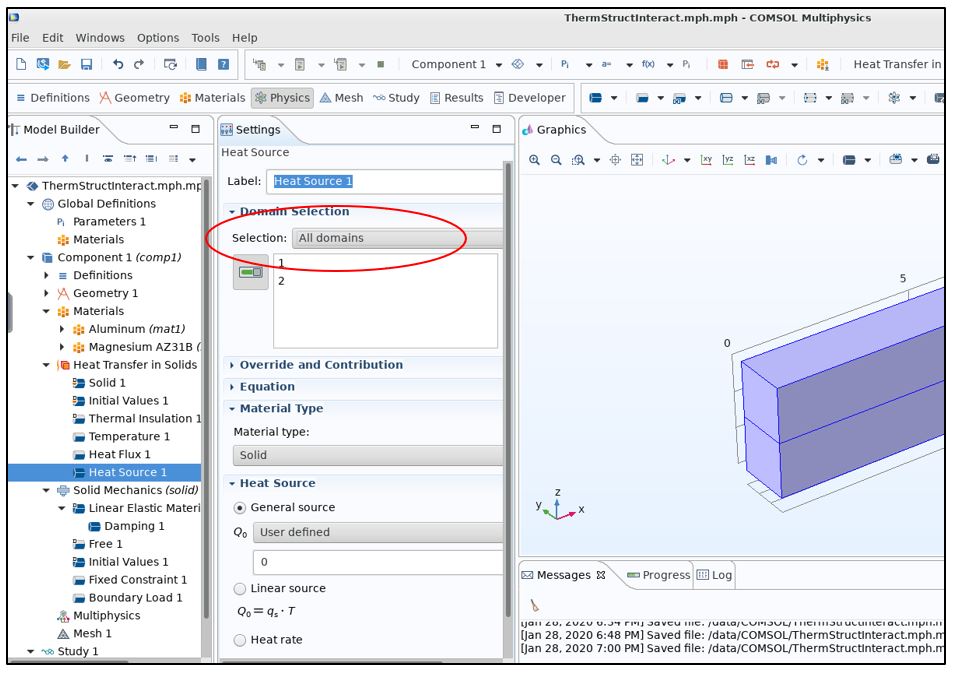
38. In the Physics toolbar, click Domains and select Heat Source and under Domain selection, select All domains as shown below:
39. Under Heat Source, choose Total power dissipation density (solid/lemm1). This selection permits the heat generation given by the vibrations in the structure.
40. The next step will be to perform the meshing of the system. Under Model Builder to Component 1 (comp1), click Mesh 1. In the Mesh settings, locate the Physics-Controlled Mesh.
41. Select Element size as Extra fine.
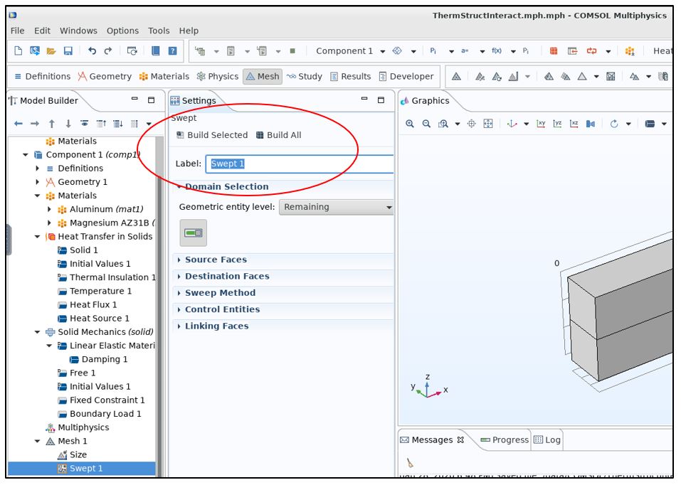
42. Right-click on Component 1(comp 1) to Mesh 1 and select Swept and then click Build All, as shown below:
43. Under Model Builder à Study 1 to click Step 1: Time Dependent, as shown below:
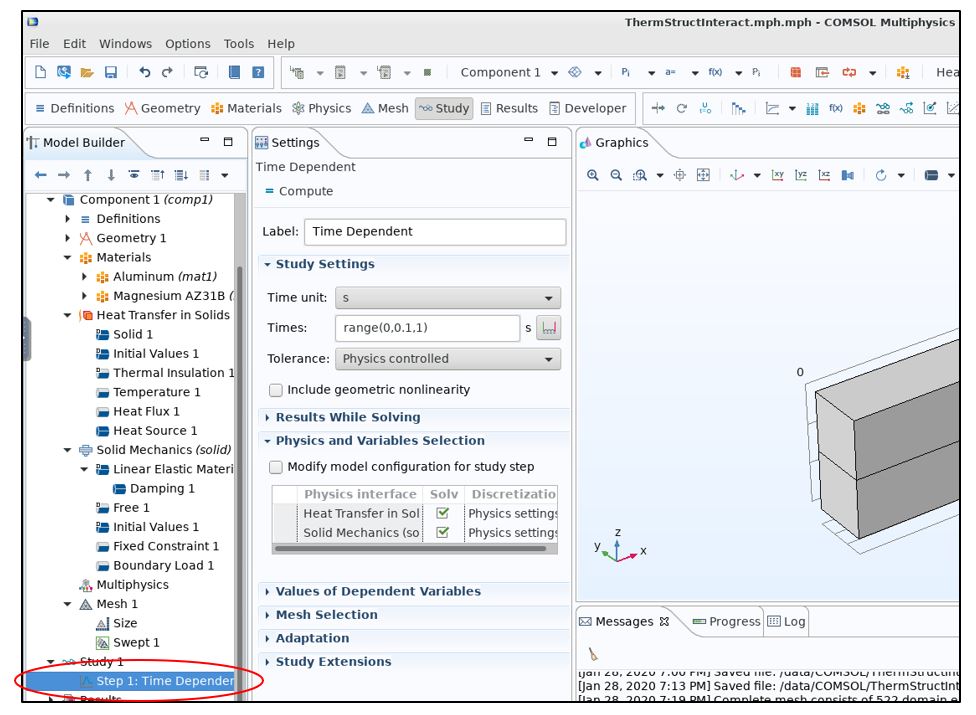
44. Under Study Settings to Times, type: 0, 0.05, and 2.
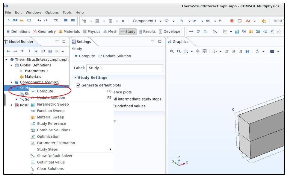
45. Right-click on Study 1 and choose Get Initial Value.
46. In this step, we will generate some results by going to Model Builder and expanding Temperature (ht) and select Surface.
47. Under Settings for Surface, go to Expression and type T-293.15 to get the temperature in degrees C.
48. In the Model Builder, under Study 1, select Step 1: Time Dependent and under the Settings, click on the Results While Solving, so expand this section. Select the Plot checkbox.
NOTE: Some detailed images showing the steps above were purposely skipped to keep the case study shorter and to the scope.
49. In the Model Builder under Study 1, select Solver Configurations. Click Solver Configurations to expand and then select Solution 1 (sol 1). Choose Time-Dependent Solver 1 as shown below (you must enable manually the complex values because we need to use them in the solid mechanics equations):
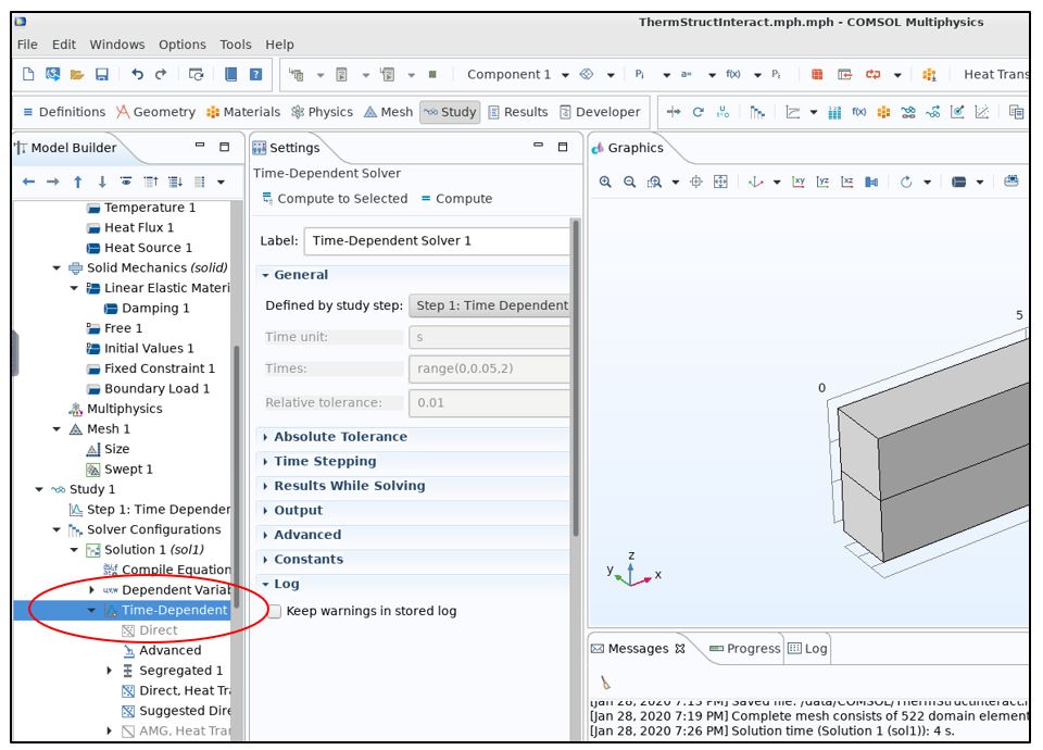
50. Under Time-Dependent Solver, click Advanced to expand and select Allow complex numbers.
51. Go to Home and click Compute.
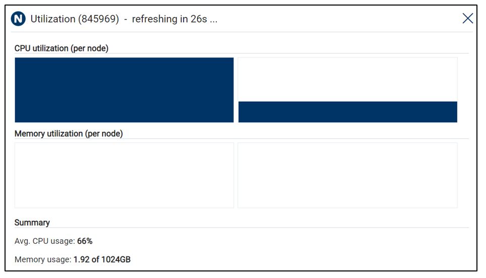
52. Monitor your CPU utilization (Click “Detailed Job Metrics” to see the utilization of your nodes during Solve):
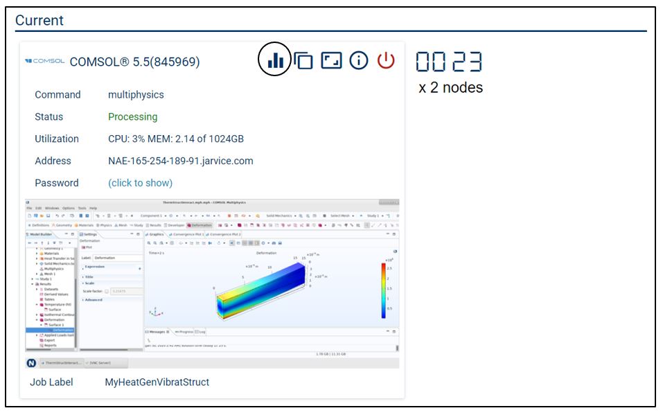
NOTE: The CPU utilization time refreshes every 30 seconds. For distributed problems, all nodes will be displayed along with CPU utilization per node.
53. Insert and review your results (select results as desired in the “Model Builder” view/tab under “Results”) as shown below:
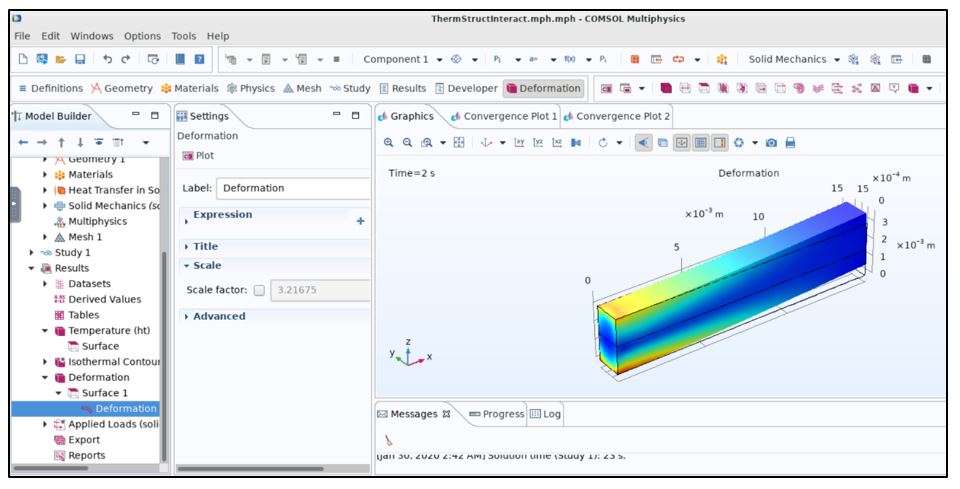
Structural Results
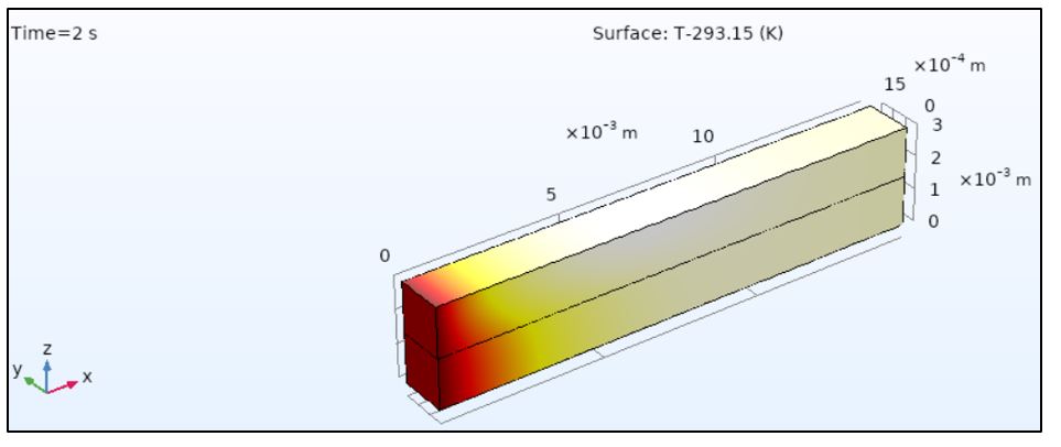
Thermal Results
54. Save and Exit once post-processing is completed.